I looked at quite some different approaches to the Fibonacci function, and I start to wonder how the Fibonacci number develops with respect to its index. To look into this I want to make a 2D plot where the X-axis is the natural numbers and the Y-axis is the corresponding Fibonacci numbers.

To solve this problem I decided to use R. This is less of an obvious solution. Usually one would probably have gone for a spreadsheet, but already did that.

R is a good tool for doing numeric analysis and prototyping algorithms for machine learning. For that it provides good tools for visualizing data. This is what I am going to elaborate a bit on here.

Day 8 - R

Usually I would have started implementing Fibonacci as a recursive function. This was also my first approach and it is certainly possible. It is, however, not the idiomatic way. R is an array oriented language and as such we work on arrays. Under this paradigm it is better to initialize an array, and then populate it with its elements.

The implementation takes offset in a function that takes n as input and returns a list of the n first Fibonacci numbers.

fibList <- function(n){  theList <- numeric(n)  theList[1] <- 1  theList[2] <- 1  for (i in 3:n) {    theList[i] <- theList[i-1] + theList[i-2]  }  return(theList);}# Calling the functionfibList(10)fibList(20)fibList(100)

It was run using the Rscript command

mads@mads:fibonacci$ Rscript fib.R  [1]  1  1  2  3  5  8 13 21 34 55 [1]    1    1    2    3    5    8   13   21   34   55   89  144  233  377  610[16]  987 1597 2584 4181 6765  [1] 1.000000e+00 1.000000e+00 2.000000e+00 3.000000e+00 5.000000e+00  [6] 8.000000e+00 1.300000e+01 2.100000e+01 3.400000e+01 5.500000e+01 [11] 8.900000e+01 1.440000e+02 2.330000e+02 3.770000e+02 6.100000e+02 [16] 9.870000e+02 1.597000e+03 2.584000e+03 4.181000e+03 6.765000e+03 [21] 1.094600e+04 1.771100e+04 2.865700e+04 4.636800e+04 7.502500e+04 [26] 1.213930e+05 1.964180e+05 3.178110e+05 5.142290e+05 8.320400e+05 [31] 1.346269e+06 2.178309e+06 3.524578e+06 5.702887e+06 9.227465e+06 [36] 1.493035e+07 2.415782e+07 3.908817e+07 6.324599e+07 1.023342e+08 [41] 1.655801e+08 2.679143e+08 4.334944e+08 7.014087e+08 1.134903e+09 [46] 1.836312e+09 2.971215e+09 4.807527e+09 7.778742e+09 1.258627e+10 [51] 2.036501e+10 3.295128e+10 5.331629e+10 8.626757e+10 1.395839e+11 [56] 2.258514e+11 3.654353e+11 5.912867e+11 9.567220e+11 1.548009e+12 [61] 2.504731e+12 4.052740e+12 6.557470e+12 1.061021e+13 1.716768e+13 [66] 2.777789e+13 4.494557e+13 7.272346e+13 1.176690e+14 1.903925e+14 [71] 3.080615e+14 4.984540e+14 8.065155e+14 1.304970e+15 2.111485e+15 [76] 3.416455e+15 5.527940e+15 8.944394e+15 1.447233e+16 2.341673e+16 [81] 3.788906e+16 6.130579e+16 9.919485e+16 1.605006e+17 2.596955e+17 [86] 4.201961e+17 6.798916e+17 1.100088e+18 1.779979e+18 2.880067e+18 [91] 4.660047e+18 7.540114e+18 1.220016e+19 1.974027e+19 3.194043e+19 [96] 5.168071e+19 8.362114e+19 1.353019e+20 2.189230e+20 3.542248e+20

When the number is large enough R converts the list into floating point numbers. This conversion is mostly OK when working with probabilities, but can be fatal when we need the exact result. In above example the last element has been cropped. R reports 354224800000000000000 while the 100th number is 354224848179261915075.

The type conversion does not matter when visualizing. It won't even mean a pixel when plotted on the screen, so we will continue on and try to visualize the relationship between $n$ and $fib(n)$.

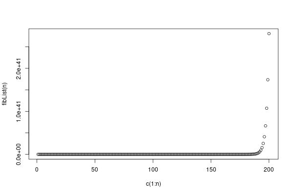
The relationship looks much like an exponential development. This, however, is a subject for a later article.

Conclusion

I implemented the recursive edition of the Fibonacci algorithm in R. This algorithm is efficient, and R provides efficient subroutines for handling the array.

After the implementation a simple plot of the relationship between $n$ and $fib(n)$ was plotted. This was easily done in R, as R provides good abstractions for this.